3  Finding the Results

Running commands in R will produce three main types of output: text, plots, and data objects.

3.1 Text Results

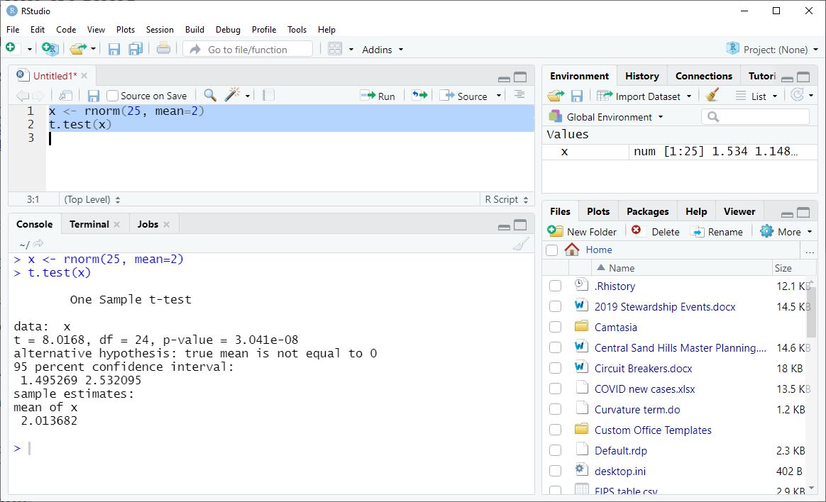
Examining text results is pretty obvious: output from R statements is “printed” to the Console by default.

We can use the output of a t-test as an example.

x <- rnorm(25, mean=2)
t.test(x)

You can resize your Console pane to see more (or less) of your output at once. The width of your Console affects where the lines of print output break, so adjust this before you run your commands.

The Console is a “buffer” that only holds 1000 lines of output. With a huge amount of output, you cannot scroll back to the beginning. For longer projects, you should save your results as data objects, which is discussed in the next chapter.

3.2 Plots

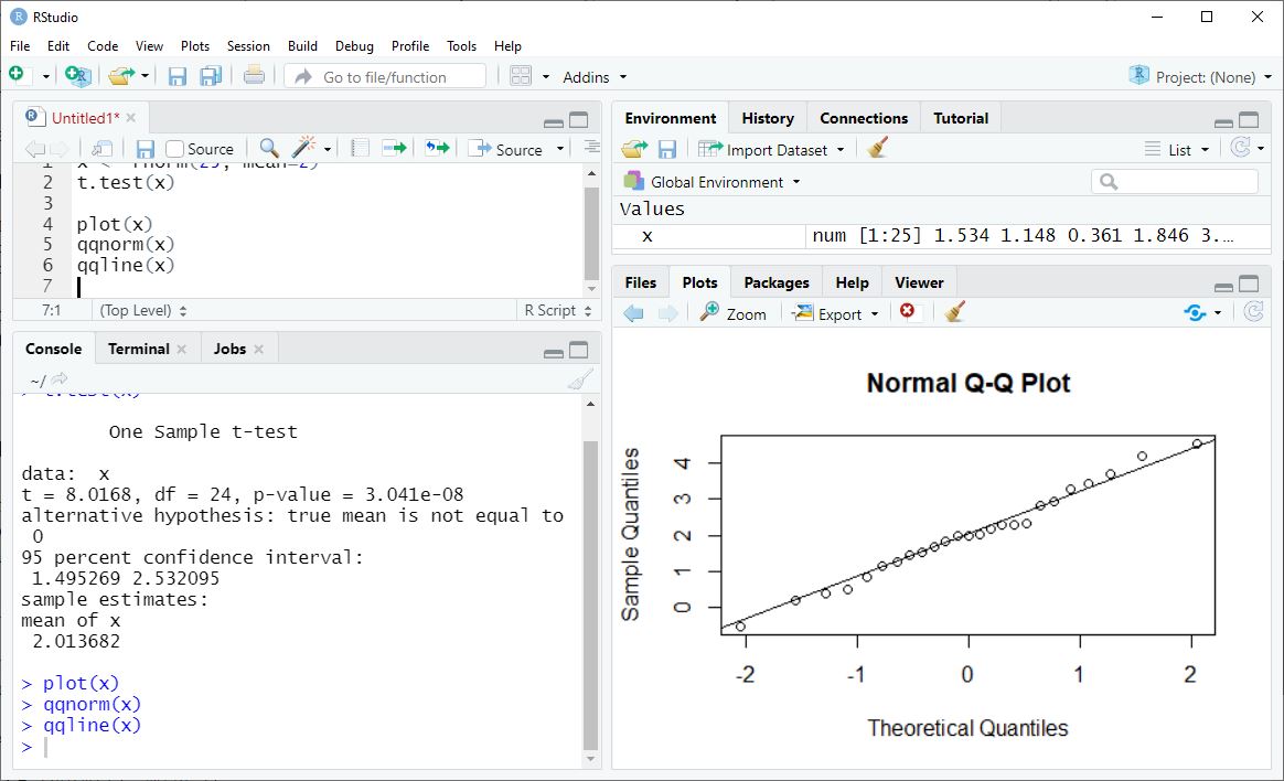
Plots appear in the Plots pane, in the lower-right corner of the RStudio workspace.

Plot the data from our last exercise as an example. Each of the first two lines below produces a plot, and the third line with qqnorm() modifies the second plot by adding a line.

plot(x)
qqnorm(x)
qqline(x)

Like the Console, the Plots pane can be resized. This changes the look of the plot (the size and the aspect ratio). You can also pop a plot into a separate window with the Zoom button in the Plots toolbar.

If you have created more than one plot, you can use the left and right arrows in the Plots toolbar to scroll among your plots.

3.3 Examining Data

Looking at data values is a little more complicated, because data comes in many forms in R. We will discuss the varieties of R data in more depth later, but for now there are three main strategies for examining data values and properties: the Environment pane, printing data to the Console, and viewing dataframes and lists.

3.3.1 Environment Pane

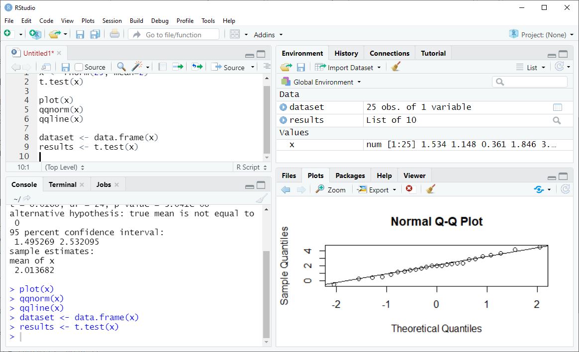
The Environment pane in the upper-right corner of the RStudio workspace shows the names of any data objects currently available in your computer’s memory.

As examples, let’s save our x data as a dataframe, and also save our t.test() results as data.

x <- rnorm(25, mean=2)
dataset <- data.frame(x)
results <- t.test(x)

In the Environment pane we see that x is a numeric vector (num) with 25 observations ([1:25]), and we can see a few of the data values. For more complicated objects like dataset and results, we can click on the blue arrow next to the name to see more details of what is inside each object, including some data values. The main thing we get out of the Environment pane is metadata, information about how each data object is defined.

3.3.2 Viewing Dataframes and Lists

If we click on the name of a dataframe or list object in the Environment pane, a tab opens in the Source pane of RStudio. For a dataframe this gives us a spreadsheet-like view of the data values. For a list, it gives us a somewhat cleaner way to browse the metadata.

3.3.3 Printing Data

For basic data objects, printing them will show us the data values. To see just a few of the data values, we can use the head() or tail() functions, which give the first or last six values or rows by default.

head(x)

[1] 0.8888263 2.9273293 1.6102052 3.4609974 2.0608079 2.2075981

head(dataset)

          x
1 0.8888263
2 2.9273293
3 1.6102052
4 3.4609974
5 2.0608079
6 2.2075981

tail(x)

[1] 2.522563 1.075333 2.109782 2.659170 2.020728 4.405015

tail(dataset)

          x
20 2.522563
21 1.075333
22 2.109782
23 2.659170
24 2.020728
25 4.405015

How an object is printed depends on its class. The head() and tail() functions printed x and dataset differently, even though these two contain the same values. Some functions handle these different object classes differently, and these are called generic functions. Click here to learn more about data structures and class.

Printing a data object like results gives us formatted output, and it does not simply show the data elements it stores. Compare this output to what we saw when we viewed results by clicking on its name in the environment.

results

    One Sample t-test

data:  x
t = 10.638, df = 24, p-value = 1.45e-10
alternative hypothesis: true mean is not equal to 0
95 percent confidence interval:
 1.716832 2.543383
sample estimates:
mean of x 
 2.130107 

3.4 Exercises

Run the following code. What type of output does each line produce? What patterns can you find in the code that helps you predict what kind of output it will produce?

x <- rnorm(100)
boxplot(x)
y <- rnorm(100, mean = 1)
t.test(x, y)
plot(x, y)
x - y